

Analysis: Is There an Ideal Production Budget?
August 30, 2012
Update: The link to the data was broken, I've corrected it.
A common area of debate for independent film-makers revolves around the question of the "ideal" production budget. Depending on who you talk to, and when, you'll hear that it's impossible to make money in the industry with a film budgeted at under $2 million, or over $10 million, or less than $20 million (or some other number). Producers who attend panels at conferences and film festivals often come back to me afterwards and ask if their $8 million project is doomed because a speaker declared that "no-one in their right mind would make an independent film for more than $5 million," or something similar.
This debate prompts a question: Is there an ideal budget for a feature film -- some budget level that will produce greater-than-expected returns for the film-maker?
In theory, answering that question should be fairly straightforward. First, we can make the simplifying assumption that domestic box office is a reasonable proxy for financial performance. Then we can look at our database of production budgets and box office results for each film, and see if there's some budget level that produces consistently higher box office returns.
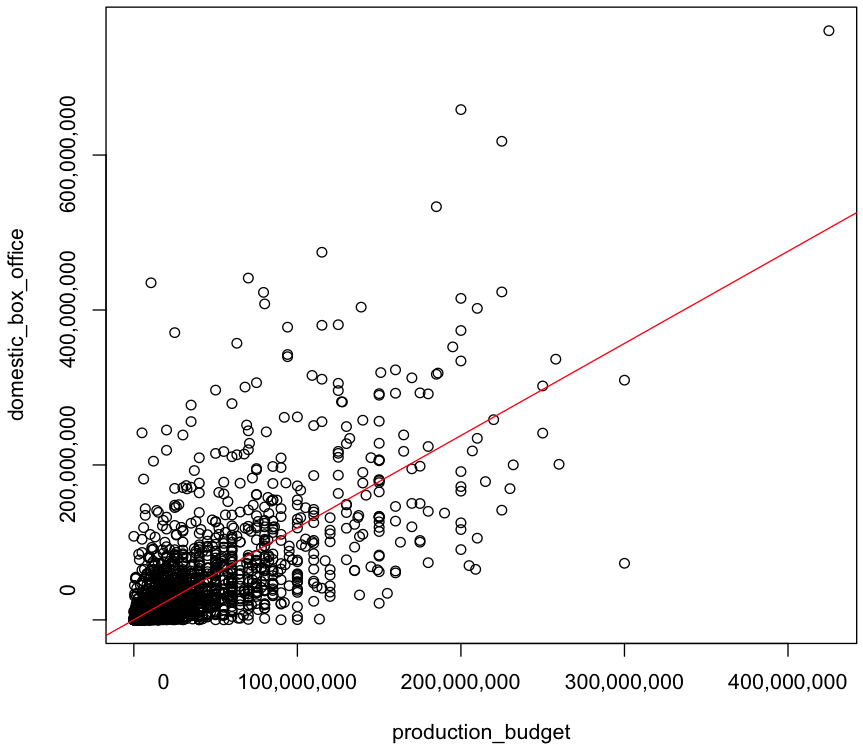
Running a linear regression using all films released in the last ten years for which we have budget and box office information (with my trusty copy of R -- non statisticians feel free to ignore the code, by the way), I get the following:
Although the graph is a bit of a mess, there is a fairly good correlation between budget and box office -- a higher budget generally leads to a higher box office. In fact, R2 is 63%, meaning that about 63% of the variance in the box office result for a film is determined by the production budget (with the other 37% presumably determined by other factors, like the relative quality of the film, the abilities of the distributor, and so on -- topics I will return to in future articles).
Having said that, one glance at the graph tells us that we'll need to do some more work to decipher an "ideal budget." There's simply too much noise for a clear pattern to be visible. To dig that out, we need to find the signal.
One way to do that is to group films with similar budgets together, see what the "typical" box office would be for films in that budget range, and then compare these typical values across the full range of budgets. For example, we could select all films with budgets between $2 million and $3 million, and then find what's typical by calculating the median box office for those films. (The advantage of using the median is that it avoids having the numbers skewed because one film in the set happens to be a massive box office hit.) Then we can do the same for films budgeted between $3 million and $4 million, and so on, and look at whether there are budget ranges that typically produce a higher box office than neighboring budgets.
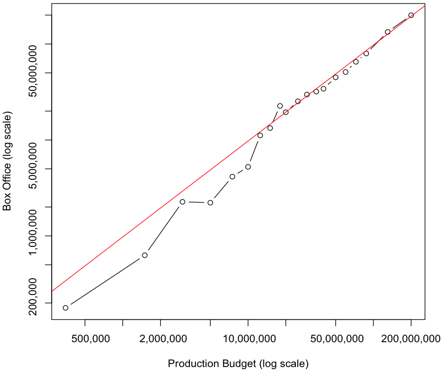
In the chart below, I've taken this approach, selecting the budget ranges by putting films in groups of 100: first the 100 least-expensive films to make, then the next 100, and so on, through to the most expensive films made in recent years. For each group, I've plotted the median box office for films in that budget range. Since we have budgets for 1,954 films, I've ended up with 20 sets of films (the last of which has 54 films). So all of the points are clear on the chart, I've plotted it using a log scale.
If there is an ideal budget, it will show itself with a point substantially above the line of best fit. And, to be honest, you'd have to squint pretty hard to see one. The biggest outlier is the range centered on an $18 million budget. That particular group has a median box office of $22,616,503, or 126% of budget. But that really looks like random noise to me. There are some dips and humps in the chart that one could interpret as meaningful -- films budgeted under $10 million seem to do a little worse than films budgeted over $10 million, for example. But there doesn't seem to be some part of the chart that rises significantly above the surrounding area.
So can we write off the idea of ideal budgets? Well, for the general case I think we can: no single production budget confers an advantage over any other, based on this analysis. But there are some other factors to consider. For example, the most expensive films in our list are almost all studio-financed projects, while the least expensive films are almost all independently-produced. There may be a transition point where independent films do horribly at the box office but the effects of that are hidden by the good performance of studio-produced films (in fact, studio-produced films may account for the modest increase in performance around the $10 million budget range). Similarly, particular genres might have budgetary sweet spots that we can't see (because, maybe, $5 million romantic comedies do badly, but $5 million horror films do quite well). That's the kind of analysis we do for our clients all the time, and we've certainly seen budget ranges that perform better or worse for particular types of film. But absent that level of analysis, the numbers tell a simple story: there's no ideal budget for a feature film.
Bruce Nash bruce.nash@the-numbers.com

> bbo <- read.csv("https://widget.opusdata.com/obqqlmdiq.csv")
> attach(bbo)
> lr <- lm(domestic_box_office~0+production_budget)
> summary(lr)

Call:
lm(formula = domestic_box_office ~ 0 + production_budget)

Residuals:
       Min         1Q     Median         3Q        Max
-283760097  -17165597   -2603363   11703828  422621897

Coefficients:
                  Estimate Std. Error t value Pr(>|t|)
production_budget  1.18940    0.02053   57.93   <2e-16 ***
---
Signif. codes:  0 ‘***’ 0.001 ‘**’ 0.01 ‘*’ 0.05 ‘.’ 0.1 ‘ ’ 1

Residual standard error: 52660000 on 1953 degrees of freedom
Multiple R-squared: 0.6321,	Adjusted R-squared: 0.6319
F-statistic:  3356 on 1 and 1953 DF,  p-value: < 2.2e-16

> plot(production_budget,domestic_box_office, xaxt="n", yaxt="n")
> axis(1,axTicks(1), format(axTicks(1), scientific = F, big.mark=","))
> axis(2,axTicks(2), format(axTicks(2), scientific = F, big.mark=","))
> abline(lr, col="red")
> production_budget[2000] <- NA
> pbm <- matrix(production_budget,100,20)
> domestic_box_office[2000] <- NA
> bom <- matrix(domestic_box_office,100,20)
> x <- apply(pbm,2,function(x) median(x,na.rm=TRUE))
> y <- apply(bom,2,function(x) median(x,na.rm=TRUE))
> lrs <- lm(y~0+x)
> summary(lrs)

Call:
lm(formula = y ~ 0 + x)

Residuals:
     Min       1Q   Median       3Q      Max
-7382042 -3992413 -1163995   202467  6832653

Coefficients:
  Estimate Std. Error t value Pr(>|t|)
x  0.97389    0.01381   70.52   <2e-16 ***
---
Signif. codes:  0 ‘***’ 0.001 ‘**’ 0.01 ‘*’ 0.05 ‘.’ 0.1 ‘ ’ 1

Residual standard error: 3944000 on 19 degrees of freedom
Multiple R-squared: 0.9962,	Adjusted R-squared: 0.996
F-statistic:  4973 on 1 and 19 DF,  p-value: < 2.2e-16

> plot(x,y, xaxt="n", yaxt="n", type="b", log="xy",
       xlab="Production Budget (log scale)", ylab="Box Office (log scale)")
> abline(lrs, untf=TRUE, col="red")
> axis(1,axTicks(1), format(axTicks(1), scientific = F, big.mark=","))
> axis(2,axTicks(2), format(axTicks(2), scientific = F, big.mark=","))
Filed under: Analysis